Mesh generation§
While not directly part of the collision detection problem, mesh generation is
useful to extend the range of shapes supported by ncollide by discretizing
them such that they can be approximated with a TriMesh, a Polyline, a
ConvexHull, and/or a Compound. It is also useful to obtain a
renderer-compliant representation of non-polyhedral models such that balls,
capsules, parametric surfaces, etc. The two main types of mesh generators
output are TriMesh and Polyline.
Triangle mesh§
The TriMesh structure describes a triangle mesh with optional per-vertex
normals and texture coordinates:
| Field | Description |
|---|---|
coords |
The vertex coordinates. |
normals |
The vertex normals. |
uvs |
The vertex texture coordinates. |
indices |
The triangles vertices index buffer. |
The index buffer may take two forms. In its UnifiedIndexBuffer form, the
index of a triangle vertex is the same as the index identifying its normal and
texture coordinates. This implies that the coordinate, normals and texture
coordinate buffers should have the same size. While not very memory-efficient,
this is the required representation for renderers based on, e.g., OpenGL. In
the following figure, each disc corresponds to one index (i.e. one integer) and
each square to one buffer element:

In its SplitIndexBuffer form, each triangle vertex as three indices: one
for its position, one for its normal, and one for its texture coordinate. This
representation is usually topologically more interesting than the unified
index buffer. In the following figure, each disc corresponds to one index
that identifies the type of element that shares the same color:

It is possible (but time-consuming) to switch between those two kinds of index buffers:
| Method | Description |
|---|---|
.unify_index_buffer() |
Transforms the current TriMesh index buffer to a UnifiedIndexBuffer. This copies the relevant data in order to make sure that every attributes of a single vertex is accessible using the same index. |
.split_index_buffer(heal) |
Transforms the current TriMesh index buffer to a SplitIndexBuffer. If heal is set to true it will attempt to recover the original mesh topology, identifying with the same index vertices having the exact same position. |
The simplest way to build a TriMesh from most primitive shapes defined by
ncollide is to import the ToTriMesh trait and call the corresponding
method.
| Method | Description |
|---|---|
.to_trimesh(...) |
Creates a polyhedral representation of self. |
This method requires a parameter that allows you to control the discretization
process. The exact type of this parameter depends on the type that implements
the trait. For example, a Ball requires two integers (one for the number of
subdivisions of each spherical coordinate) to be transformed to a TriMesh;
the Cuboid however requires a parameter equal to () because it does not
need any user-defined information in order to be discretized.
Polygonal line§
The Polyline is a much simpler data structure than the TriMesh. It does not
have an index nor texture coordinates buffer:
| Field | Description |
|---|---|
coords |
The vertex coordinates. |
normals |
The vertex normals. |
Since it does not have an index buffer coords is assumed to be a line strip,
and there is no way to let two different vertices share the same normal in
memory. This structure is not very practical to model complex 2D shapes. That
is why it should be changed to a more traditional index-buffer based
representation in future versions of ncollide.
The simplest way to build a Polyline from most primitive shapes defined by
ncollide is to import the Polyline trait and call the corresponding
method.
| Method | Description |
|---|---|
.to_polyline(...) |
Creates a polylineical representation of self. |
This method requires a parameter that allows you to control the discretization
process. The exact type of this parameter depends on the type that implements
the trait. For example, a Ball requires one integer (for the number of
subdivisions) to be transformed to a TriMesh; the Cuboid however requires a
parameter equal to () because it does not need any user-defined information
in order to be discretized.
Paths§
Path-based mesh generation exposed by the procedural::path module allows you
to create more complex 3D shapes by replicating a pattern along a path. Note
that this feature is still extremely immature and at most incomplete. Use with
care.
The path-based mesh generation API is based on two traits. The CurveSampler
trait is implemented by a structure that is capable of generating a path, i.e.,
a set of points assumed to form a polyline:
| Method | Description |
|---|---|
.next() |
Returns the next point of the path. |
The returned point may be either a StartPoint, an InnerPoint or an
EndPoint. If EndOfSample is returned, then the path generation is assumed
to be completed. There may be several pairs of StartPoint, InnerPoint inside
of the same path. This allows patterns like dashed lines.
Together with the path, we need the pattern that will be replicated at each
point of the path. Such pattern must implement the StrokePattern trait.
| Method | Description |
|---|---|
stroke(path) |
Strokes the path using self as the pattern. |
The stroke pattern is responsible for the mesh generation itself. It has to
duplicate its pattern at each point of the path, and to link those duplicates
correctly to form a topologically sound TriMesh. This allows you to easily
stroke paths with possibly very different shapes and connectivity using the
same pattern.
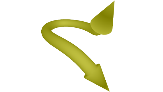
The following example uses the PolylinePath together with the
PolylinePattern to stroke the arrowed Bézier curve shown at the beginning of
this section.
let control_points = [
    Point3::new(0.0f32, 1.0, 0.0),
    Point3::new(2.0, 4.0, 2.0),
    Point3::new(2.0, 1.0, 4.0),
    Point3::new(4.0, 4.0, 6.0),
    Point3::new(2.0, 1.0, 8.0),
    Point3::new(2.0, 4.0, 10.0),
    Point3::new(0.0, 1.0, 12.0),
    Point3::new(-2.0, 4.0, 10.0),
    Point3::new(-2.0, 1.0, 8.0),
    Point3::new(-4.0, 4.0, 6.0),
    Point3::new(-2.0, 1.0, 4.0),
    Point3::new(-2.0, 4.0, 2.0),
];

// Setup the path.
let bezier = procedural::bezier_curve(&control_points, 100);
let mut path = PolylinePath::new(&bezier);

// Setup the pattern.
let start_cap = ArrowheadCap::new(1.5, 2.0, 0.0);
let end_cap = ArrowheadCap::new(2.0, 2.0, 0.5);
let pattern = ncollide2d::procedural::unit_circle(100);
let mut pattern = PolylinePattern::new(pattern.coords(), true, start_cap, end_cap);

// Stroke!
let _ = pattern.stroke(&mut path);
Mesh transformation§
Meshes can be computed from other meshes as well. This may be useful to make them usable by some geometric queries that have specific requirements. For example most queries on ncollide require the objects to be convex or to be the union of several convex objects. A convex hull or a convex decomposition may thus help to pre-process complex concave meshes.
Convex Hull§
Besides the ToTriMesh and ToLinestrip traits, the procedural and
transformation modules export free functions that generate various meshes and
line strips, including those accessible by the two former traits.
It also exposes functions to compute the convex hull of a set of point using the QuickHull algorithm which has an average O(nlogn) time complexity:
| Function | Description |
|---|---|
convex_hull(...) |
Computes the convex hull of a set of points. |
If you are not interested in the Polyline representation of the 2D convex
hull but only on the original indices of the vertices it contains, use the
_idx variant of the function − namely convex_hull2d_idx(...).
The following example creates 100,000 random points and compute their
convex hull.
let mut points = Vec::new();
for _ in 0usize..100000 {
    points.push(rand::random::<Point3<f32>>() * 2.0);
}

let _ = transformation::convex_hull(&points[..]);
let mut points = Vec::new();
for _ in range(0u, 100000) {
points.push(rand::random::<Point3<f32>>() * 2.0f32);
}
let convex_hull = transformation::convex_hull(&points[..]);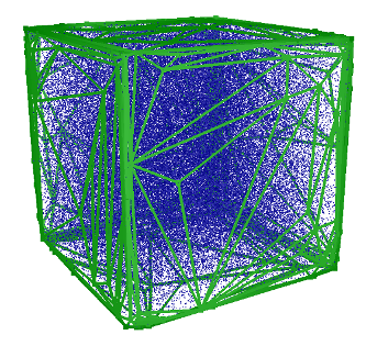
Convex decomposition§
While convex objects
have nice properties that help designing efficient algorithms, studies show
that using only convex objects leads to very boring applications! That is why
ncollide allows the description of concave objects from its convex parts
using the Compound shape. For example, one could describe the following
object as the union of two convex parts:

But decomposing manually a concave polyhedra into its convex parts is a very tedious task and computing an exact convex decomposition is often not necessary. That is why ncollide implements the 3D HACD algorithm that computes an approximate convex decomposition. It is not yet implemented in 2D.
HACD§
The HACD is simply a clustering algorithm based on a concavity criterion to separate the different groups. It will group triangles together until the directional distances between their vertices and their convex hull do not exceed an user-defined limit.
To compute the decomposition of a triangle mesh, use the procedural::hacd
function. It takes three arguments:
| Argument | Description |
|---|---|
mesh |
The TriMesh to decompose. It must have normals. Disconnected components of the mesh will not be merged together. |
error |
The maximum normalized concavity per cluster. It must not be close to a limit value like Bounded::max_value(). Values around 0.03 seems to give fine results for most objects. |
min_components |
Force the algorithm not to generate more than min_components convex parts. |
Let us define what normalized concavity means. Because there is no official definition of the concavity of a 3D object, we are using the maximal distance between the triangle mesh vertices and its convex hull. This distance is computed along the direction of the vertex normal (hence, it is usually different from the intuitive distance obtained by orthogonal projection of the point on the closest convex hull face):

Then, to make this concavity measure kind of independent from the whole shape dimensions, it is divided by the object AABB diagonal D:

We call the ratio dD the normalized concavity. In this example, it is equal to 6.010.0=0.6.
The procedural::hacd function returns a tuple. Its first member is the set of
convex objects that approximate the input mesh and the second one is the set of
indices of the triangles used to compute each convex object.
The following figure shows a tube (left), the result of the clustering done by the HACD algorithm (middle), and the resulting approximate convex decomposition (right):
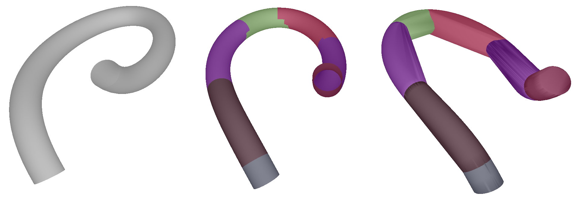
The following example creates a concave object using a path-based mesh generation and approximates it using the HACD algorithm. Together with kiss3d, this code was used to generate the figure above.
let control_points = [
    Point3::new(0.0f32, 1.0, 0.0),
    Point3::new(2.0, 4.0, 2.0),
    Point3::new(2.0, 1.0, 4.0),
    Point3::new(4.0, 4.0, 6.0),
    Point3::new(2.0, 1.0, 8.0),
    Point3::new(2.0, 4.0, 10.0),
    Point3::new(0.0, 1.0, 12.0),
    Point3::new(-2.0, 4.0, 10.0),
    Point3::new(-2.0, 1.0, 8.0),
    Point3::new(-4.0, 4.0, 6.0),
    Point3::new(-2.0, 1.0, 4.0),
    Point3::new(-2.0, 4.0, 2.0),
];
let bezier = procedural::bezier_curve(&control_points, 100);
let mut path = PolylinePath::new(&bezier);
let pattern = ncollide2d::procedural::unit_circle(100);
let mut pattern = PolylinePattern::new(pattern.coords(), true, NoCap::new(), NoCap::new());
let mut trimesh = pattern.stroke(&mut path);

// The path stroke does not generate normals =(
// Compute them as they are needed by the HACD.
trimesh.recompute_normals();

/*
  * Decomposition of the mesh.
  */
let (decomp, partitioning) = transformation::hacd(trimesh.clone(), 0.03, 0);

// We end up with 7 convex parts.
assert!(decomp.len() == 7);
assert!(partitioning.len() == 7);
Collision detection pipeline Miscellaneous